Regression Analysis in Excel Chart
After you plot your data in say XY type graph, you can also get the regression line directly from the graph. Here is the procedure
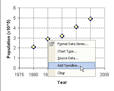
1. I assume you already have the data and plot it in XY type. Suppose the data is only five points of populations in 20 years gathered every 5 consecutive years as shown in the figure below.
2. Click on any data point. Then do Right click and pop up menu will appear. Select Add Trendline
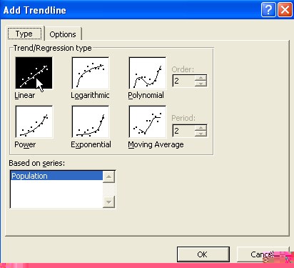
3. Add Trendline dialog will appear. Select Linear Trend/Regression type.
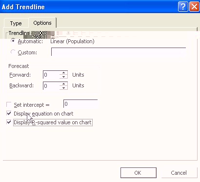
4. Go to Options Tab by clicking on it. Check Display Equation on Chart and Display R-squared value on chart then click OK button.
5. The results of regression line as well as the regression equation model and the R-squared value will appear on the chart.
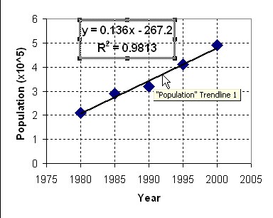
This trend line is quite dynamic. If you change your data, the trend line (and the regression equation) will also change automatically.
<
Previous
|
Next
|
Content
>
Send your comments, questions and
suggestions
Preferable reference for this tutorial is
Teknomo, Kardi (2015) Regression Model using Microsoft Excel. http://people.revoledu.com/kardi/tutorial/Regression/