By Lyra Filiola

Bootstrap Statistics for Generalized Linear Regression
In this section we will performs Bootstrap for general linear regression model (or so called Multiple Linear regression model). You can input as many independent variables as you want. Note that the independent variable should have been a matrix with the first column filled by "1".
For example:
 > x1<-1:10


 > x2<-11:20


 > x3<-21:30


 > x<-matrix(1,10)


 > x<-cbind(x,x1,x2,x3)


 > x


   x1 x2 x3


   [1,] 1 1 11 21


   [2,] 1 2 12 22


   [3,] 1 3 13 23


   [4,] 1 4 14 24


   [5,] 1 5 15 25


   [6,] 1 6 16 26


   [7,] 1 7 17 27


   [8,] 1 8 18 28


   [9,] 1 9 19 29


   [10,] 1 10 20 30


 >
In this section we will discuss about the script I made to perform Boostrap on general linear regression model. Similar to previous section, the script is separated part by part and the explanation of each part of the script will follow after that. Later, you can see some example application on how to use this script using R. The script itself can be downloaded here.
The Bootstrap's script for general linear regression case is as follows:
  I multiple.reg.boot<-function(x,y,p,b,k,alpha)


   {


II n<-length(y)


   int1<-t(x)


   int2<-int1%*%x


   int3<-solve(int2)


   int4<-int1%*%y


   koef.beta<-int3%*%int4


   index.beta<-matrix(0:(p-1))


   out<-cbind(index.beta,koef.beta)


   cat("Least Square Estimator","\n")


   print(out)
cat("\n") III cat("Standard Error for Beta","\n") int5<-t(y) int6<-t(koef.beta) int7<-int5%*%y int8<-int6%*%int1 int9<-int8%*%y sse<-int7-int9 mse<-sse/(n-p) msedata<-mse[1] var.all<-msedata*int3 var.koef.beta<-diag(var.all) se.koef.beta<-sqrt(var.koef.beta) print(se.koef.beta) cat("\n")IV cat(((1-(alpha))*100),"% Confidence Interval for Beta","\n") low<-koef.beta-qt((1-(alpha/2)),(n-p))*se.koef.beta up<-koef.beta+qt((1-(alpha/2)),(n-p))*se.koef.beta cat("Lower Bound","\n") print(low) cat("\n") cat("Upper Bound","\n") print(up) cat("\n")V matcoef<-matrix(0:(p-1)) beta.boot=NULL for(i in 1:b) { VI v<-sample(1:n,k,replace=TRUE) ystarpre<-y[v] xstarpre<-x[v,1:p] ystar<-data.matrix(ystarpre) xstar<-data.matrix(xstarpre) inta<-t(xstar) intb<-inta%*%xstar detb<-det(intb)VII if(detb==0) { repeat { v<-sample(1:n,k,replace=TRUE) ystarpre<-y[v] xstarpre<-x[v,1:p] ystar<-data.matrix(ystarpre) xstar<-data.matrix(xstarpre) inta<-t(xstar) intb<-inta%*%xstar detb<-det(intb) if(detb!=0) next } }VIII intc<-solve(intb) intd<-inta%*%ystar koef.beta.boot<-intc%*%intd { beta.boot=koef.beta.boot } matcoef<-cbind(matcoef,beta.boot) }IX matcoef1<-matcoef[,2:(b+1)] mean.beta.boot<-apply(matcoef1,1,mean) bias.beta.boot<-mean.beta.boot-koef.beta var.beta.boot<-apply(matcoef1,1,var) se.beta.boot<-sqrt(var.beta.boot)loboundpre<-matrix(0:(p-1)) upboundpre<-matrix(0:(p-1)) for (t in 1:p) { matquant<-matcoef1[t,] loboundquant<-quantile(matquant,(alpha/2)) upboundquant<-quantile(matquant,(1-(alpha/2)))loboundpre<-rbind(loboundpre,loboundquant) upboundpre<-rbind(upboundpre,upboundquant) }lobound0<-loboundpre[(p+1):(2*p),] upbound0<-upboundpre[(p+1):(2*p),]lobound<-matrix(0:(p-1)) lobound<-cbind(lobound,lobound0)upbound<-matrix(0:(p-1)) upbound<-cbind(upbound,upbound0)X cat("Bootstrap Correlation Model","\n") cat("bias beta","\n") print(bias.beta.boot) cat("\n") cat("standard error beta","\n") print(se.beta.boot) cat("\n") cat((1-alpha)*100,"% Confidence Interval for beta","\n") cat("lower bound =","\n") print(lobound) cat("upper bound =","\n") print(upbound) cat("\n")}
Next I will explain the script above part by part
Part I
This program named "
multiple.reg.boot
" and the inputs are as follows:
x : matrix of independent variable
y : matrix of dependent variable
p : number column of x
b : number of Bootstrap's replications
k : length of Bootstrap sample
alpha : significance level
Part II
This part is calculating regression's estimator using least square method.
Part III
This part calculates the standard error for estimator of regression.
Part IV
This part calculates the confidence interval for estimator of regression.
Part V
This part is the beginning of Bootstrapping. First, we define matcoef and Bootstrap estimator for regression, beta.boot. Those statistics will be bootstrapped.
Part VI
This part obtains Bootstrap sample.
Part VII
This part anticipates if the determinant of is equal to 0, so that the inverse is not defined. In this part, syntax at part VI is repeated until it finds such Bootstrap sample that the determinant of is not equal to 0.
Part VIII
This part is the finishing of Bootstrapping data. The result is stored at a matrix named matcoef.
Part IX
Remember in part V, matcoef defined as certain matrix and then it is added by Bootstrap estimator of regression. For the next computation, we don't need the first column in matcoef. So, matcoef1 is defined as matcoef without the first column. The bias, standard error and confidence interval is computed here.
Part X
This part sets the output of bootstrapping data.
Example:
To see how the script works, we use the data set about "Zarthan Company" taken from Neter (1990).
Dataset is divided into independent variable and dependent variable. For this case, "Target Population" and "Per Capita Discretionary Income" are the independent variable, and "Sales" is the dependent variable.
> y


   [1] 162 120 223 131 67 169 81 192 116 55 252 232 144 103 212


 > x


   x1 x2


   [1,] 1 274 2450


   [2,] 1 180 3254


   [3,] 1 375 3802


   [4,] 1 205 2838


   [5,] 1 86 2347


   [6,] 1 265 3782


   [7,] 1 98 3008


   [8,] 1 330 2450


   [9,] 1 195 2137


   [10,] 1 53 2560


   [11,] 1 430 4020


   [12,] 1 372 4427


   [13,] 1 236 2660


   [14,] 1 157 2088


   [15,] 1 370 2605


 >
Suppose you have save the script in directory name " D:/MyDirectory ", then you can load this script into R with the following command
> source("D:/MyDirectory/multipleregboot.R")
Alternatively you can use menu File > Source R code... and pointing to the script file.
To use the data set above for Boostrap general linear regression model, you type
> multiple.reg.boot(x,y,3,500,15,0.1)
The command above will generate 15 Bootstrap samples, each sample has 500 replication from the orginal data set that has independent variable name x and dependent variable name y with 10% significant level. The independent variables contain 3 columns. The result of this computation is as follows:
Least Square Estimator


   [,1] [,2]


   0 3.45261279


   x1 1 0.49600498


   x2 2 0.00919908
Standard Error for Beta


   x1 x2


   2.4306504935 0.0060544412 0.0009681139
90 % Confidence Interval for Beta


           Lower Bound


   [,1]


   -0.879505337


   x1 0.485214221


   x2 0.007473624
Upper Bound


   [,1]


   7.78473092


   x1 0.50679573


   x2 0.01092454
Bootstrap Correlation Model


           bias beta


   [,1]


   -8.032102e-02


   x1 -3.723742e-04


   x2 1.598148e-05
standard error beta


   x1 x2


   3.026618419 0.005882961 0.001164328
90 % Confidence Interval for beta


           lower bound =


   lobound0


   loboundquant 0 -1.78008148


   loboundquant 1 0.48541920


   loboundquant 2 0.00719702
upper bound =


   upbound0


   upboundquant 0 8.76600905


   upboundquant 1 0.50505110


   upboundquant 2 0.01119679
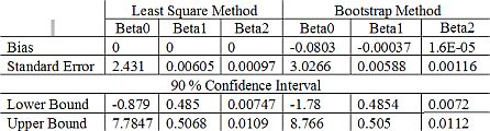
The output above shows that Bootstrap also did a good job in estimating the property of general linear regression's estimators. The result from Bootstrap method is not differ very much from the classical method. Table below show some comparison between Bootstrap method and Classical Least square method.
REFERENCES
Dalgaard, P. (2002). Introductory Statistics with R. New York: Springer.
Efron, B. and Tibishirani, R. J. (1993). An Introduction to the Bootstrap. London�: Chapman & Hall.
Greene, W. H. (2000). Econometric Analysis. New York: Macmillan Publishing Company.
Neter, J., and friends. (1990). Applied Linear Statistical Models: Regression, Analysis of Variance, and Experimental Designs, Third Edition. Boston: Irwin.
R Development Core Team (2006). R: A language and environment for statistical computing. R Foundation for Statistical Computing, Vienna, Austria. ISBN 3-900051-07-0, URL http://www.R-project.org.
This tutorial is copyrighted .
Preferable reference for this tutorial is
Filiola, L., (2006) Bootstrap Computation using R, http://people.revoledu.com/kardi/tutorial/Bootstrap/Lyra/index.html