
<
Previous
|
Next
|
Contents
>
Read this tutorial comfortably off-line, click here to purchase the e-book of this AHP tutorial.
AHP Numerical Example
In this section, I show an example of two levels AHP. The structure of hierarchy in this example can be drawn as the following
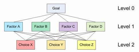
Level 0 is the goal of the analysis. Level 1 is multi criteria that consist of several factors. You can also add several other levels of sub criteria and sub-sub criteria but I did not use that here. The last level (level 2 in figure above) is the alternative choices. You can see again Table 1 for several examples of Goals, factors and alternative choices. The lines between levels indicate relationship between factors, choices and goal. In level 1 you will have one comparison matrix corresponds to pair-wise comparisons between 4 factors with respect to the goal. Thus, the comparison matrix of level 1 has size of 4 by 4. Because each choice is connected to each factor, and you have 3 choices and 4 factors, then in general you will have 4 comparison matrices at level 2. Each of these matrices has size 3 by 3. However, in this particular example, you will see that some weight of level 2 matrices are too small to contribute to overall decision, thus we can ignore them.
Based on questionnaire survey or your own paired comparison, we make several comparison matrices. Click here if you do not remember how to make a comparison matrix from paired comparisons. Suppose we have comparison matrix at level 1 as table below. The yellow color cells in upper triangular matrix indicate the parts that you can change in the spreadsheet. The diagonal is always 1 and the lower triangular matrix is filled using formula
![]() .
.
Table 9: Paired comparison matrix level 1 with respect to the goal
|
Criteria |
A |
B |
C |
D |
Priority Vector |
|
A |
1.00 |
3.00 |
7.00 |
9.00 |
57.39% |
|
B |
0.33 |
1.00 |
5.00 |
7.00 |
29.13% |
|
C |
0.14 |
0.20 |
1.00 |
3.00 |
9.03% |
|
D |
0.11 |
0.14 |
0.33 |
1.00 |
4.45% |
|
Sum |
1.59 |
4.34 |
13.33 |
20.00 |
100.00% |
![]() =4.2692, CI = 0.0897, CR = 9.97% < 10% (acceptable)
=4.2692, CI = 0.0897, CR = 9.97% < 10% (acceptable)
The priority vector is obtained from normalized Eigen vector of the matrix. Click here if you do not remember how to compute priority vector and largest Eigen value
![]() from a comparison matrix. CI and CR are consistency Index and Consistency ratio respectively, as I have explained in previous section. For your clarity, I include again here some part of the computation:
from a comparison matrix. CI and CR are consistency Index and Consistency ratio respectively, as I have explained in previous section. For your clarity, I include again here some part of the computation:
![]()
![]()
![]() (Thus, OK because quite consistent)
(Thus, OK because quite consistent)
Random Consistency Index (RI) is obtained from Table 8.
Suppose you also have several comparison matrices at level 2. These comparison matrices are made for each choice, with respect to each factor.
Table 10: Paired comparison matrix level 2 with respect to Factor A
|
Choice |
X |
Y |
Z |
Priority Vector |
| X | 1.00 | 1.00 | 7.00 | 51.05% |
| Y | 1.00 | 1.00 | 3.00 | 38.93% |
| Z | 0.14 | 0.33 | 1.00 | 10.01% |
| Sum | 2.14 | 2.33 | 11.00 | 100.00% |
![]() =3.104, CI = 0.05, CR = 8.97% < 10% (acceptable)
=3.104, CI = 0.05, CR = 8.97% < 10% (acceptable)
Table 11: Paired comparison matrix level 2 with respect to Factor B
|
Choice |
X |
Y |
Z |
Priority Vector |
|
X |
1.00 |
0.20 |
0.50 |
11.49% |
|
Y |
5.00 |
1.00 |
5.00 |
70.28% |
|
Z |
2.00 |
0.20 |
1.00 |
18.22% |
|
Sum |
8.00 |
1.40 |
6.50 |
100.00% |
![]() =3.088, CI = 0.04, CR = 7.58% < 10% (acceptable)
=3.088, CI = 0.04, CR = 7.58% < 10% (acceptable)
We can do the same for paired comparison with respect to Factor C and D. However, the weight of factor C and D are very small (look at Table 9 again, they are only about 9% and 5% respectively), therefore we can assume the effect of leaving them out from further consideration is negligible. We ignore these two weights as set them as zero. So we do not use the paired comparison matrix level 2 with respect to Factor C and D. In that case, the weight of factor A and B in Table 9 must be adjusted so that the sum still 100%
Adjusted weight for factor A =
![]()
Adjusted weight for factor B =
![]()
Then we compute the overall composite weight of each alternative choice based on the weight of level 1 and level 2. The overall weight is just normalization of linear combination of multiplication between weight and priority vector.
![]()
![]()
![]()
Table 12: Overall composite weight of the alternatives
|
|
Factor A |
Factor B |
Composite Weight |
|
(Adjusted) Weight |
0.663 |
0.337 |
|
|
Choice X |
51.05% |
11.49% |
37.72% |
|
Choice Y |
38.93% |
70.28% |
49.49% |
|
Choice Z |
10.01% |
18.22% |
12.78% |
For this example, we get the results that choice Y is the best choice, followed by X as the second choice and the worst choice is Z. The composite weights are ratio scale. We can say that choice Y is 3.87 times more preferable than choice Z, and choice Y is 1.3 times more preferable than choice X.
We can also check the overall consistency of hierarchy by summing for all levels, with weighted consistency index (CI) in the nominator and weighted random consistency index (RI) in the denominator. Overall consistency of the hierarchy in our example above is given by
 (Acceptable)
Final Remark
By now you have learned several introductory methods on multi criteria decision making (MCDM) from simple cross tabulation, using rank, and weighted score until AHP. Using Analytic Hierarchy Process (AHP), you can convert ordinal scale to ratio scale and even check its consistency.
<
Previous
|
Next
|
Contents
>
Read this tutorial in a nice PDF format, click here to purchase the e-book of this AHP tutorial.
Do you have question regarding this AHP tutorial? Ask your question here
These tutorial is copyrighted .
Preferable reference for this tutorial is
Teknomo, Kardi. (2006) Analytic Hierarchy Process (AHP) Tutorial .
http://people.revoledu.com/kardi/tutorial/AHP/