Q-Learning Numerical Example

by Kardi Teknomo

<Contents | Previous | Next >

To understand how the Q learning algorithm works, we will go through several steps of numerical examples. The rest of the steps can be can be confirm using the program (you can freely download either MS Excel or Matlab code companion of this tutorial)

Let us set the value of learning parameter and initial state as room B.

First we set matrix Q as a zero matrix.

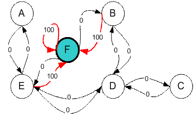
I put again the instant reward matrix R that represents the environment in here for your convenience.

Look at the second row (state B) of matrix R. There are two possible actions for the current state B, that is to go to state D, or go to state F. By random selection, we select to go to F as our action.

Now we consider that suppose we are in state F. Look at the sixth row of reward matrix R (i.e. state F). It has 3 possible actions to go to state B, E or F.

Since matrix Q that is still zero, are all zero. The result of computation is also 100 because of the instant reward.

The next state is F, now become the current state. Because F is the goal state, we finish one episode. Our agent's brain now contain updated matrix Q as

For the next episode, we start with initial random state. This time for instance we have state D as our initial state.

Look at the fourth row of matrix R; it has 3 possible actions, that is to go to state B, C and E. By random selection, we select to go to state B as our action.

Now we imagine that we are in state B. Look at the second row of reward matrix R (i.e. state B). It has 2 possible actions to go to state D or state F. Then, we compute the Q value

We use the updated matrix Q from the last episode. and . The result of computation because of the reward is zero. The Q matrix becomes

The next state is B, now become the current state. We repeat the inner loop in Q learning algorithm because state B is not the goal state.

For the new loop, the current state is state B. I copy again the state diagram that represent instant reward matrix R for your convenient.

There are two possible actions from the current state B, that is to go to state D, or go to state F. By lucky draw, our action selected is state F.

Now we think of state F that has 3 possible actions to go to state B, E or F. We compute the Q value using the maximum value of these possible actions.

The entries of updated Q matrix contain are all zero. The result of computation is also 100 because of the instant reward. This result does not change the Q matrix.

Because F is the goal state, we finish this episode. Our agent's brain now contain updated matrix Q as

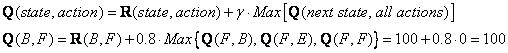
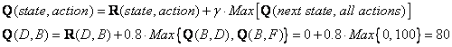
If our agent learns more and more experience through many episodes, it will finally reach convergence values of Q matrix as

This Q matrix, then can be normalized into a percentage by dividing all valid entries with the highest number (divided by 500 in this case) becomes

Once the Q matrix reaches almost the convergence value, our agent can reach the goal in an optimum way. To trace the sequence of states, it can easily compute by finding action that makes maximum Q for this state.

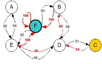
For example from initial State C, it can use the Q matrix as follow:

From State C the maximum Q produces action to go to state D

From State D the maximum Q has two alternatives to go to state B or E. Suppose we choose arbitrary to go to B

From State B the maximum value produces action to go to state F

Thus the sequence is C – D – B – F

<Contents | Previous | Next >

This tutorial is copyrighted.

Preferable reference for this tutorial is

Teknomo, Kardi. 2005. Q-Learning by Examples. http://people.revoledu.com/kardi/tutorial/ReinforcementLearning/index.html