Bootstrap Sampling Tutorial: simple linear regression

Bootstrap Sampling Tutorial

Bootstrap Statistics for Simple Linear Regression

Another usage of Bootstrap is to estimate the property of the estimator of regression model's parameter. There are at least 2 ways to do Bootstrap regression. First method is to resample the observation (correlation model). Second method is to perform resampling of the residual (residual model). In this section of tutorial, I will perform the correlation model in obtaining the property of beta-zero and beta-one.

First I will discuss about the script I made to perform Boostrap on simple linear regression case. You can download the R-script in here . For the shake of clarity, the script is separated part by part and the explanation of each part of the script follows after that. Then, you can see some example on how to use this script using R.

The Bootstrap's function for simple linear regression is as follows:

I simp.reg.boot<-function(x,y,b,k,alpha)



             {



             II n<-length(x)



             a1<-data.frame(x,y)



             a<-data.matrix(a1)

III inta<-n*sum(x*y)



             intb<-sum(x)*sum(y)



             intc<-n*sum(x^2)



             intd<-(sum(x))^2



             inte<-inta-intb



             intf<-intc-intd



             beta1<-inte/intf



             ybar<-sum(y)/n



             xbar<-sum(x)/n



             beta0<-ybar-(beta1*xbar)

IV cat("Least Square Method","\n")



             cat("beta zero =",beta0,"\n")



             cat("beta one =",beta1,"\n")

V yhat<-beta0+(beta1*x)



             mse<-sum((y-yhat)^2)/(n-2)



             varbeta1<-mse/sum((x-xbar)^2)



             sebeta1<-sqrt(varbeta1)



             sxx<-sum((x-xbar)^2)



             varbeta0<-mse*(sum(x^2)/(n*sxx))



             sebeta0<-sqrt(varbeta0)

 cat("Classical Method","\n")



             VI cat("The accuracy of beta zero","\n")



             cat("bias of beta zero =",0,"\n")



             cat("standard error of beta zero =",sebeta0,"\n")



             cat(((1-alpha)*100),"% confidence interval for beta zero","\n")



     lslobound0=beta0-(qt(1-(alpha/2),(n-2))*sebeta0)



     lsupbound0=beta0+(qt(1-(alpha/2),(n-2))*sebeta0)

 cat("lower bound =",lslobound0,"\n")



             cat("upper bound =",lsupbound0,"\n")



             cat("\n")

VII cat("The accuracy of beta one","\n")



             cat("bias of beta one =",0,"\n")



             cat("standard error of beta one =",sebeta1,"\n")



             cat(((1-alpha)*100),"% confidence interval for beta one","\n")



     lslobound1=beta1-(qt(1-(alpha/2),(n-2))*sebeta1)



     lsupbound1=beta1+(qt(1-(alpha/2),(n-2))*sebeta1)

 cat("lower bound =",lslobound1,"\n")



             cat("upper bound =",lsupbound1,"\n")



             cat("\n")

VIII bootbeta0=NULL



       bootbeta1=NULL



       IX for(i in 1:b)



       {



       X v<-sample(1:n,k,replace=TRUE)



       indep<-a[v]



       dep<-a[v,2]



       int1<-k*sum(indep*dep)



       int2<-sum(indep)*sum(dep)



       int3<-k*sum(indep^2)



       int4<-(sum(indep))^2



       int5<-int1-int2



       int6<-int3-int4



       betaboot1<-int5/int6



       depbar<-sum(dep)/k



       indepbar<-sum(indep)/k



       betaboot0<-depbar-(betaboot1*indepbar)



       {



       XI bootbeta0[i]=betaboot0



       bootbeta1[i]=betaboot1



       }



       }

 cat("\n")



             cat("Bootstrap for Regression, Correlation Model","\n")

XII meanbetaboot0=mean(bootbeta0)



             cat("Bootstrap's beta zero :",meanbetaboot0,"\n")



             cat("The Bootstrap's accuracy measures of beta zero","\n")



     biasbeta0=meanbetaboot0-beta0



     cat("bootstrap's bias for beta zero=",biasbeta0,"\n")

XIII varbetaboot0=var(bootbeta0)



       sebetaboot0=sqrt(varbetaboot0)



       cat("bootstrap's standard error for beta zero=",sebetaboot0,"\n")

XIV cat(((1-alpha)*100),"% confidence interval for beta zero","\n")



       lobound0=quantile(bootbeta0,(alpha/2))



       upbound0=quantile(bootbeta0,(1-(alpha/2)))

 cat("lower bound =",lobound0,"\n")



             cat("upper bound =",upbound0,"\n")

 cat("\n")

XV meanbetaboot1=mean(bootbeta1)



             cat("Bootstrap's beta one :",meanbetaboot1,"\n")



             cat("The Bootstrap's accuracy measures of beta one","\n")



     biasbeta1=meanbetaboot1-beta1



     cat("bootstrap's bias for beta one=",biasbeta1,"\n")

XVI varbetaboot1=var(bootbeta1)



       sebetaboot1=sqrt(varbetaboot1)



       cat("bootstrap's standard error for beta one=",sebetaboot1,"\n")

XVII cat(((1-alpha)*100),"% confidence interval for beta one","\n")



       lobound1=quantile(bootbeta1,(alpha/2))



       upbound1=quantile(bootbeta1,(1-(alpha/2)))

 cat("lower bound =",lobound1,"\n")



             cat("upper bound =",upbound1,"\n")

XVIII par(mfrow=c(1,2))



       hist(bootbeta0)



       hist(bootbeta1)



       }

Now I will explain the code above part by part.

Part I
This program named " simp.reg.boot " and needs several inputs as follows:
x : independent variable
y : dependent variable
b : number of Bootstrap replication
k : length of Bootstrap sample
alpha : significance level

Part II
This part is a preparation for data. The "a1" is data formed as frame, and "a" is "a1" assigned as matrix.

Part III
This section performs the computing of beta zero and beta one by using least square method.

Part IV
This section sets the output to perform the value of beta zero and beta one .

Part V
This section performs the computing of several properties that needed for next steps.

Part VI
This section performs the computation and the output setting for the accuracy measures of beta zero, which are its bias, standard error, and confidence interval.

Part VII
This part is more like previous part (part VI), but this one is about beta-one .

Part VIII
This part is the preparation for Bootstrap replication. We want to get the properties of beta-zero by obtaining Bootstrap's beta-zero and Bootstrap's beta-one which named as bootbeta0 and bootbeta1 , respectively. Before the Bootstrap replication begins, bootbeta0 and bootbeta1 need to be assigned as null.

Part IX
This part is the expression for b Bootstrap replications.

Part X
This part contains the resample process. First, we define the index that we need to assign the observation into Bootstrap sample. The index named as "v". For each Bootstrap sample, calculate estimator of beta0 and estimator beta1 , which named as betaboot0 and betaboot1 respectively, using the mechanism of least square method. Then, we have those estimators for each bootstrap sample.

Part XI
The estimators of beta-zero and beta-one for Bootstrap sample is assigned as bootbeta0 and bootbeta1 , respectively, which we have assigned as null in the first place.

Part XII, XIII, XIV
This part shows the computing of Bootstrap's bias, standard error, and confidence interval for beta-zero .

Part XV, XVI, XVII
This part shows the computing of Bootstrap's bias, standard error, and confidence interval for beta-one .

Part VIII
First, this part sets the form of graph's output. We want to see the histogram of bootbeta0 and bootbeta1 in one window. And the syntax is as written in this part.

Example
In order to see how the script works, we will use the data set about "Disposable Personal Income and Personal Consumption Expenditures in US, 1970-1979" taken from Greene, (2000). This dataset is divided into independent variable and dependent variable. For this case, income is the independent variable, and consump is the dependent variable.

> income
[1] 751.6 779.2 810.3 864.7 857.5 874.9 906.8 942.9 988.8 1015.7
> consump
[1] 672.1 696.8 737.1 767.9 762.8 779.4 823.1 864.3 903.2 927.6

Suppose you have save the script in directory name " D:/MyDirectory ", then you can load this script into R with the following command

> source("D:/MyDirectory/simp.reg.boot.R")

Alternatively you can use menu File > Source R code... and pointing to the script file.

Now to use the data set above for Boostrap simple linear regression, you type

> simp.reg.boot(income,consump,500,10,0.1)

That command will generate 10 Bootstrap samples, each sample has 500 replication from the orginal data set that has independent variable name income and dependent variable name consump with 10% significant level. The output is shown below

Least Square Method
beta zero = -67.58065
beta one = 0.979267
Classical Method
The accuracy of beta zero
bias of beta zero = 0
standard error of beta zero = 27.91071
90 % confidence interval for beta zero
lower bound = -119.4820
upper bound = -15.67935

The accuracy of beta one
bias of beta one = 0
standard error of beta one = 0.03160707
90 % confidence interval for beta one
lower bound = 0.920492
upper bound = 1.038042

Bootstrap for Regression, Correlation Model
Bootstrap's beta zero : -68.33979
The Bootstrap's accuracy measures of beta zero
bootstrap's bias for beta zero= -0.759142
bootstrap's standard error for beta zero= 25.31215
90 % confidence interval for beta zero
lower bound = -111.1430
upper bound = -37.03275

Bootstrap's beta one : 0.979773
The Bootstrap's accuracy measures of beta one
bootstrap's bias for beta one= 0.0005060599
bootstrap's standard error for beta one= 0.02806356
90 % confidence interval for beta one
lower bound = 0.942392
upper bound = 1.025886
>

bootstrap histogram

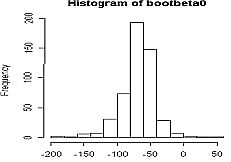
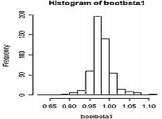
The output above shows that Bootstrap did a good job in estimating the property of beta zero and beta one, because the result from Bootstrap method is not very differ from the classical method. Also, the histogram for bootbeta0 and bootbeta1 are nearly normal because of the large number of Bootstrap replication.

< Back | Next | Index >

This tutorial is copyrighted .

Preferable reference for this tutorial is

Filiola, L., (2006) Bootstrap Computation using R, http://people.revoledu.com/kardi/tutorial/Bootstrap/Lyra/index.html

Bootstrap for Simple Linear Regression

Bootstrap Statistics for Simple Linear Regression