<
Previous
|
Next
|
Contents
>
What is Kernel Regression?
Kernel regression is an estimation technique to fit your data. Given a data set
![]() , you want to find a regression function
, you want to find a regression function
![]() such that that function is best-fit match to your data at those data points. You may also want to interpolate and approximate a little bit beyond your data.
such that that function is best-fit match to your data at those data points. You may also want to interpolate and approximate a little bit beyond your data.
Different from linear regression or polynomial regression that you know the underlying assumption (e.g. normal distribution), kernel regression does not assume any underlying distribution to estimate the regression function. That is why kernel regression is categorized as non-parametric technique.
The idea of kernel regression is putting a set of identical weighted function called Kernel local to each observational data point. The kernel will assign weight to each location based on distance from the data point. The kernel basis function depend only to the radius or width (or variance) from the 'local' data point X to a set of neighboring locations x. Kernel regression is a superset of local weighted regression and closely related to Moving Average and K nearest neighbor (KNN) , radial basis function (RBF), Neural Network and Support Vector Machine (SVM).
Let us start with an example.
Suppose you have data like the following table.
|
|
1 |
2 |
3 |
4 |
5 |
|
|
1 |
1.2 |
3.2 |
4 |
5.1 |
|
|
23 |
17 |
12 |
27 |
8 |
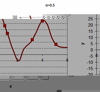
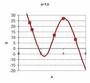
The graph of the data is shown below. It is clearly non-linear if you are sure that each data contains no-error.
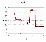
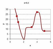
You want to obtain curve-fitting function to your data such that the result would be like one of these charts below. There are many ways to do curve fitting and Kernel regression is just one of them.
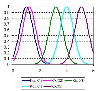
In Kernel regression, what you do is to put a kernel (a kind of bump function) to each point of your X data. The following graph shows Gaussian kernels are located in the center of each data X.
By putting the kernel at your original data
![]() , now you can extend the value of the original data
, now you can extend the value of the original data
![]() into much smaller value of
into much smaller value of
![]() at certain small step
at certain small step
![]() . For example, we use
. For example, we use
![]() (smaller is smoother). For the first data point
(smaller is smoother). For the first data point
![]() , we can sample the kernel value at each small step of
, we can sample the kernel value at each small step of
![]() .
.
The formula of Gaussian Kernel is
In this tutorial, the notation of your observational data point is
![]() , while the estimation and domain sampling points are denoted by
, while the estimation and domain sampling points are denoted by
![]() . In this simple example you have only 5 data points but you can make as many sampling points as you want by setting sampling rate
. In this simple example you have only 5 data points but you can make as many sampling points as you want by setting sampling rate
![]() .
.
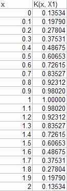
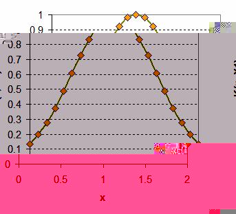
Assume that the kernel width
![]() (we talk about
kernel width later
), then we can compute the sample kernel as the following
(we talk about
kernel width later
), then we can compute the sample kernel as the following
And so on, we can put into table and chart as shown below
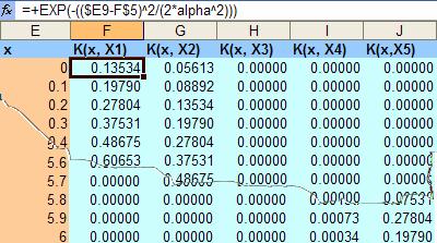
Similar procedure can be done for the all other data points
![]() . As our data points have
. As our data points have
![]() have range of 1 to 5.1, we can extend the domain of
have range of 1 to 5.1, we can extend the domain of
![]() between 0 and 6. Computing the kernel values
between 0 and 6. Computing the kernel values
![]() for each data point
for each data point
![]() of each sample of domain value
of each sample of domain value
![]() produce a table like the following:
produce a table like the following:
For your convenience, you can download the spreadsheet example of this tutorial here .
Then the estimated value of
![]() at domain value
at domain value
![]() is given by this
Kernel Regression formula
(also called
Nadaraya-Watson
kernel weighted average)
is given by this
Kernel Regression formula
(also called
Nadaraya-Watson
kernel weighted average)

The nominator of the Kernel Regression formula is array sum product of kernel and weight, while the denominator is just sum of kernel value at domain
![]() for all data point
for all data point
![]() . The following figure show the excel function formulation estimated y using for kernel regression formula for x=0
. The following figure show the excel function formulation estimated y using for kernel regression formula for x=0
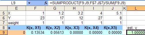
At beginning we just put all weights values as one, thus all the estimated y is also one as illustrated in the figure below. Copy the estimated y formula for all domain value x, then compute the square of error of estimated y compared to the original
![]() data.
data.
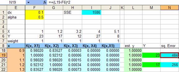
Get the sum of square or all the original data (at beginning it is quite high value, SSE= 1586 in our example). Now we are ready for the solution. To find the solution, we will use MS Excel Solver.
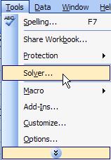
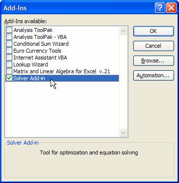
Check your Tools menu if there is no solver menu, its mean you need to install the Solver. To install the Solver, you go to menu Tools-Add-Ins... and check on the Solver Add-in and click OK button.
If you already have Solver, click that menu Tools-Solver? and you will have a solver parameters dialog
We want to find weights for each kernel that minimize the sum of square error. Set the target cell of the sum of square error ( SSE ) equal to Min by changing cells weight array. Then click Solve button and click OK button in the next Solver Results dialog to Keep Solver Solution
As we get the new weights array as solution, we also automatically solve the regression by computing the values of estimated y. Figure below shows that the sum of square error is almost zero (
![]() ).
).
Plotting all the value of domain x and estimated y we get the following chart. The dot marker is the original five data points
![]() .
.