Share this:
Google+
< Previous | Contents | Next >
Random Walk from Normal Distribution
In the previous section, we have learned that Random Walk was generated based on uniform distribution. In this section, you will learn a random walk that generated using normal distribution.
One of the simplest model is to assume the time series data are generated based on a certain probability distribution. The simplest technique is to predict the future value only based on one last value on the data. Model that only based on one last value of the data is called following Markov property. Suppose the current time series data is denoted by \(x_t \), and then the future value would be estimated as $$ x_{t+1}=x_t + \Delta x_t $$
In each time step, we draw independent random value from the given probability distribution. Thus, these random values are called to be drawn from an independent identical distribution (iid). Most often used probability distribution is a Normal Distribution.
Why we use independent Normal distribution? The independent random values represent the influence of all other variables that are not in the model. The excluded variables are unpredictable (random). A large number of small disturbances, whose effect cannot be predicted, are similar to statistical error of measurement. Though they are unpredictable, their effect can be understood through the theory of statistical error developed by Gauss. The sum of these large number of very small disturbances, approximate Normal distribution (based on Central Limit Theorem).
Let us denote a random values that is drawn from Normal probability distribution with mean \( \mu \) and standard deviation \( \sigma \) as \( N(\mu, \sigma) \).
If the random values is drawn from a Normal probability distribution with mean \( \mu=0 \) and unit standard deviation \( \sigma = 1 \) then we have what is called as white Gaussian noise \( N(0, 1) \). A random walk model with white noise is also called Brownian motion.
$$ \Delta x_t = N(0, 1) $$
To do random walk in spreadsheet such as Microsoft Excel, we can use formula of inverse of normal distribution by setting the probability as uniform distribution random number U=RAND().
$$ \Delta x_t = x_{t+1}-x_t = NORMINV(U,0,1) $$
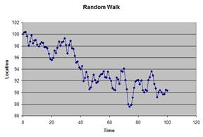
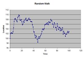
Several results are shown in the figures below. Please keep in mind that the apparent trend or apparent seasonal effects are not real because it happens only by random chance. There is no autocorrelation in the random walk model.


The spread of the distribution of the prediction is increased with the square root of the number of steps (periods of forecasting).
In the next section, you will learn how to simulate Random walk in a spreadsheet.
< Previous | Contents | Next >
Do you have question regarding this Stochastic Process tutorial? Ask your question here
These tutorial is copyrighted .
Preferable reference for this tutorial is
Teknomo, Kardi. (2019) Stochastic Process Tutorial .
http://people.revoledu.com/kardi/tutorial/StochasticProcess/

