KNN for Smoothing and Prediction

By Kardi Teknomo, PhD.

<Previous | Next | Contents>

Read it off line on any device. Click here to purchase the complete E-book of this tutorial

Using the same principle, we can extend the K-Nearest Neighbor (KNN) algorithm for smoothing (interpolation) and prediction (forecasting, extrapolation) of quantitative data (e.g. time series). In classification, the dependent variable Y is categorical data. In this section, the dependent variable has quantitative values.

Here is step by step on how to compute K-nearest neighbors KNN algorithm for quantitative data:

1. Determine parameter K = number of nearest neighbors
2. Calculate the distance between the query-instance and all the training samples
3. Sort the distance and determine nearest neighbors based on the K-th minimum distance
4. Gather the values of of the nearest neighbors
5. Use average of nearest neighbors as the prediction value of the query instance

KNN for Extrapolation, Prediction, Forecasting

Example (KNN for Extrapolation, Prediction, Forecasting)

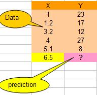
We have 5 data pair (X,Y) as shown below. The data are quantitative in nature. Suppose the data is sorted as in time series. Then the problem is to estimate the value of Y based on K-Nearest Neighbor (KNN) algorithm at X=6.5

1. Determine parameter K = number of nearest neighbors

Suppose use K = 2

2. Calculate the distance between the query-instance and all the training samples

Coordinate of query instance is 6.5. As we are dealing with one-dimensional distance, we simply take absolute value from the query instance to value of X.

For instance for X=5.1, the distance is | 6.5 – 5.1 | = 1.4, for X = 1.2 the distance is | 6.5 – 1.2 | = 5.3 and so on.

3. Sort the distance and determine nearest neighbors based on the K-th minimum distance

As the data is already sorted, the nearest neighbors are the last K data.

4. Gather the values of of the nearest neighbors

We simply copy the Y values of the last K=2 data. The result is tabulated below.

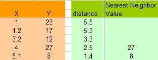
5. Use average of nearest neighbors as the prediction value of the query instance

In this case, we have prediction value of

You can play around with different data and value K if you download the spreadsheet of this example here.

KNN for Interpolation, Smoothing

Example (KNN for Interpolation)

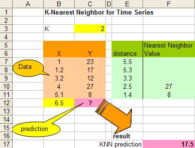
Using the same training data and the same technique, we can also do KNN for smoothing (interpolation between values). Thus, our data is shown as

Suppose we know the X data is between 0 and 6 and we would like to compute the value of Y between them.

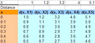
1. We define dx=0.1 and set the value of x = 0 to 6 with increment dx
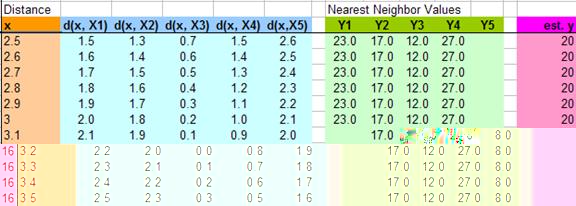
2. Compute distance between x (as if it is the query instance) and each of the data X

For instance the distance between query instance x = 0.1 and X2 = 1.2 is denoted as d(x, X2) = | 0.1 – 1.2 | = 1.1. Similarly, distance between query instance x = 0.5 and X5 = 5.1 is computed as d(x, X5) = | 0.5 – 5.1 | = 4.6. Table below shows distance for x = 0 to 0.5 for all X data

1. We obtain the nearest neighbors based on the K-th minimum distance and copy the value of Y of the nearest neighbors.
2. The smoothing estimate is the arithmetic average of the values of the nearest neighbors

Table below shows example of computation of KNN for smoothing for x = 2.5 until 3.5.

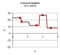
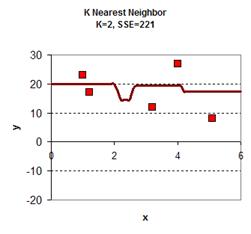
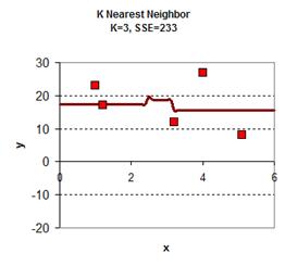
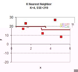
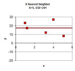
Playing around with the value of K give the graph results is give below. In general, the plot of KNN smoothing has many discontinuities. For K=1, the KNN smoothing line goes passing all the data points, therefore the sum of square error is zero. The plot is the most rough. When K = 5 (all the data point), we get only one horizontal line as the average of all data. Between the two extremes, we can find adjust the value of K as parameter to adjust the smoothing plot. Among K=2, K=3 and K=4 we obtain K=4 have the smallest sum of square error (SSE) .

download the spreadsheet of this example here

I have demonstrated through several examples how we can use simple K-NN algorithm for classification, interpolation and extrapolation.

Click here to purchase the complete E-book of this tutorial

Give your feedback and rate this tutorial

<Contents | Previous | Next >

This tutorial is copyrighted.

Preferable reference for this tutorial is

Teknomo, Kardi. K-Nearest Neighbors Tutorial. http:\\people.revoledu.com\kardi\ tutorial\KNN\