
Click here to purchase the complete E-book of this tutorial
There are several most popular decision tree algorithms such as ID3, C4.5 and CART (classification and regression trees). In general, the actual decision tree algorithms are recursive. (For example, it is based on a greedy recursive algorithm called Hunt algorithm that uses only local optimum on each call without backtracking. The result is not optimum but very fast). For clarity, however, in this tutorial, I will describe as if the algorithm is iterative.
Here is an explanation on how a decision tree algorithm work. We have a data record which contains attributes and the associated classes. Let us call this data as table D. From table D, we take out each attribute and its associate classes. If we have p attributes, then we will take out p subset of D. Let us call these subsets as Si . Table D is the parent of table Si.
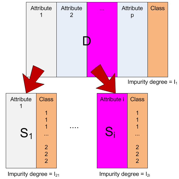
From table D and for each associated subset Si , we compute degree of impurity. We have discussed about how to compute these indices in the previous section.
To compute the degree of impurity, we must distinguish whether it is come from the parent table D or it come from a subset table Si with attribute i.
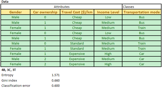
If the table is a parent table D, we simply compute the number of records of each class. For example, in the parent table below, we can compute degree of impurity based on transportation mode. In this case we have 4 Busses, 3 Cars and 3 Trains (in short 4B, 3C, 3T):
If the table is a subset of attribute table Si , we need to separate the computation of impurity degree for each value of the attribute i.

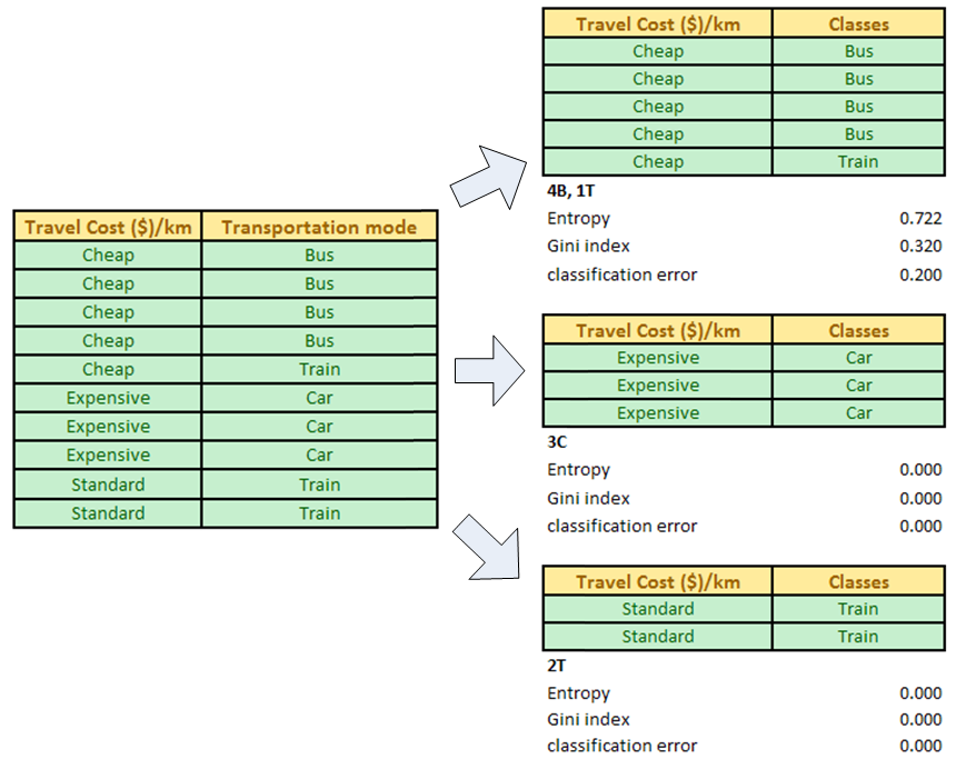
For example, attribute Travel cost per km has three values: Cheap, Standard and Expensive. Now we sort the table Si = [Travel cost/km, Transportation mode] based on the values of Travel cost per km. Then we separate each value of the travel cost and compute the degree of impurity (either using entropy, gini index or classification error).
Information gain
The reason for different ways of computation of impurity degrees between data table D and subset table Si is because we would like to compare the difference of impurity degrees before we split the table (i.e. data table D) and after we split the table according to the values of an attribute i (i.e. subset table Si) . The measure to compare the difference of impurity degrees is called information gain . We would like to know what our gain is if we split the data table based on some attribute values.
Information gain is computed as impurity degrees of the parent table and weighted summation of impurity degrees of the subset table. The weight is based on the number of records for each attribute values. Suppose we will use entropy as measurement of impurity degree, then we have:
Information gain (i) = Entropy of parent table D - Sum (n k /n * Entropy of each value k of subset table Si )
For example, our data table D has classes of 4B, 3C, 3T which produce entropy of 1.571. Now we try the attribute Travel cost per km which we split into three: Cheap that has classes of 4B, 1T (thus entropy of 0.722), Standard that has classes of 2T (thus entropy = 0 because pure single class) and Expensive with single class of 3C (thus entropy also zero).
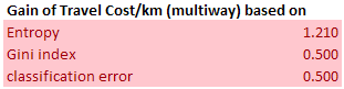
The information gain of attribute Travel cost per km is computed as 1.571 ? (5/10 * 0.722+2/10*0+3/10*0) = 1.210
You can also compute information gain based on Gini index or classification error in the same method. The results are given below.
For each attribute in our data, we try to compute the information gain. The illustration below shows the computation of information gain for the first iteration (based on the data table) for other three attributes of Gender, Car ownership and Income level.
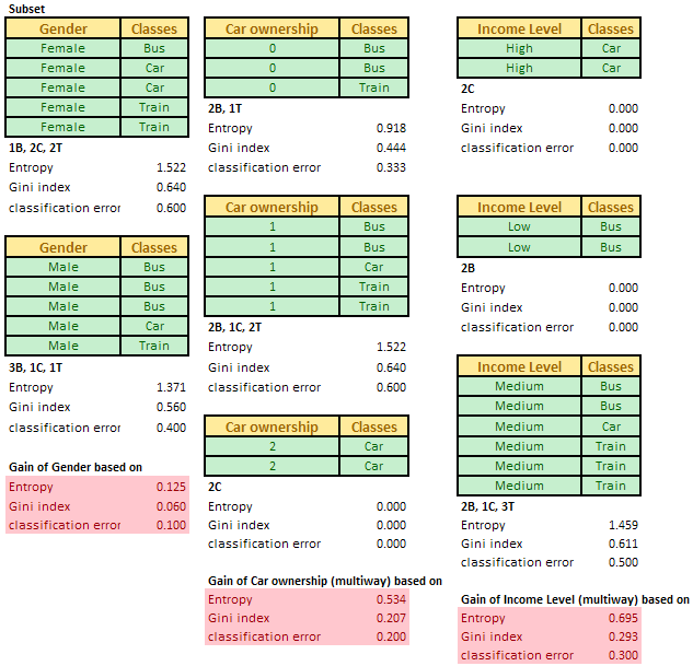
Table below summarizes the information gain for all four attributes. In practice, you don't need to compute the impurity degree based on three methods. You can use either one of Entropy or Gini index or index of classification error.
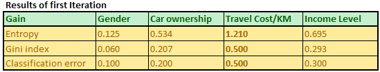
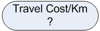
Once you get the information gain for all attributes, then we find the optimum attribute that produce the maximum information gain (i* = argmax {information gain of attribute i}). In our case, travel cost per km produces the maximum information gain. We put this optimum attribute into the node of our decision tree. As it is the first node, then it is the root node of the decision tree. Our decision tree now consists of a single root node.
Once we obtain the optimum attribute, we can split the data table according to that optimum attribute. In our example, we split the data table based on the value of travel cost per km.
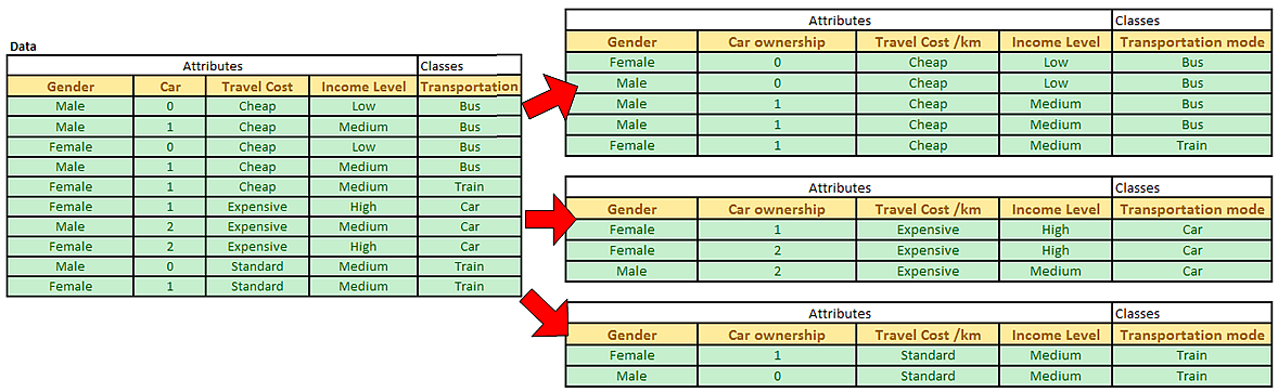
After the split of the data, we can see clearly that value of Expensive travel cost/km is associated only with pure class of Car while Standard travel cost/km is only related to pure class of Train. Pure class is always assigned into leaf node of a decision tree. We can use this information to update our decision tree in our first iteration into the following.
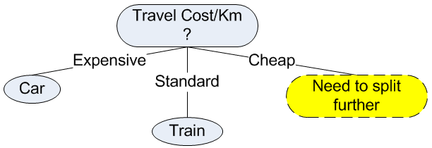
For Cheap travel cost/km, the classes are not pure, thus we need to split further in the next iteration.
Click here to purchase the complete E-book of this tutorial
This tutorial is copyrighted .
Preferable reference for this tutorial is
Teknomo, Kardi. (2009) Tutorial on Decision Tree. http://people.revoledu.com/kardi/tutorial/DecisionTree/