Bayes Rules
In learning Bayes rule or Bayes theorem, most people usually get difficulty to determine which one is a priori, posteriori, and likelihood probability. Bayes theorem itself is actually very simple. This tutorial will help you to understand Bayes theorem with an example of tabular data. If you are still confused with notation like
![]() , you may read first the
previous section of this tutorial on conditional probability
.
You can also download the spreadsheet file companion of this tutorial here.
, you may read first the
previous section of this tutorial on conditional probability
.
You can also download the spreadsheet file companion of this tutorial here.
Bayes' Rule:
![]()
-
 is called
prior
probability of our hypothesis
 . It is our state of knowledge about hypothesis
 before
we get the data
 .
.
-
 is called
likelihood
probability. It is the probability based on our observation data
 given that our hypothesis
 is hold.
-
 is the prior probability that the data
 will be observed. It is the probability of data
 without
knowledge of any hypothesis.
-
The ratio
 is called
irrelevance
index. If the irrelevance index is 1, any knowledge about B is not relevance to A. Any value below 1 measures the relevancy between A and B.
-
 is called
posterior
probability. It is our state of knowledge about hypothesis
 after
we know data
 .
.

In many applications, however, we usually have several
mutually exclusive
hypotheses
![]() . Since the data
. Since the data
![]() is a subset of our hypotheses set, we can decompose the data into
is a subset of our hypotheses set, we can decompose the data into
![]()
Because
![]() and Union operation is equivalent to summation, we obtain
and Union operation is equivalent to summation, we obtain
Total Probability Theorem :
![]()
Input the total probability theorem into Bayes' rule we get Bayes' Theorem

We use the same example as in section Conditional Probability . Refresh again your understanding about that section where you have the data and then you compute the percentage by row, percentage by column and percentage by total.
Bayes theorem problem is somewhat reversed from what we compute in section Conditional Probability . Now suppose you know only the percentage by row and the marginal percentage (from the percentage by total ), as shown in the tables below.


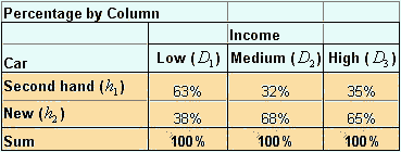
The question is: can you get the percentage by column only based on the information of these two tables?
To answer this kind of question is what the Bayes theorem help.
The two tables above can be put into notational table as follow:

And

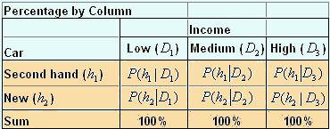
While table percentage by column , can be put into notation as table below

Using Bayes rule
![]() we can easily compute the percentage by column. For example
we can easily compute the percentage by column. For example
![]() and
and
![]() . The full table of percentage by column is presented below
. The full table of percentage by column is presented below

Send your comments, questions and suggestions
Preferable reference for this tutorial is
Teknomo, Kardi. Data Analysis from Questionnaires. https:\\people.revoledu.com\kardi\ tutorial\Questionnaire\
