Parameter Estimation of Arithmetic Brownian Motion

Share this: Google+
< Previous | Contents | Next >

Parameters Estimation in ABM

Suppose you have historical price data and you want to use Arithmetic Brownian motion model. How are you going to get the parameters of drift m and volatility s?

Recall ABM model is $ X_t=x_0+mt+sw_t $ where $ w_t \sim \sqrt{t} N(0,1) $. We input the Brownian motion, we have $ X_t=x_0+mt+s\sqrt{t} N(0,1) $. We cannot use regression model directly because of the stochastic term $ N(0,1) $.

The idea of two-steps process parameter estimation for linear model is using the analogy of finding points to determine a line. Suppose we want to find a line equation $ Y=gX+c $ from two points. What two points are the easiest to define? One is when $ X=0 $ and the other point is when $ Y=0 $ .

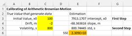
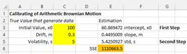
Step 1. Using similar idea, we can first assume the volatility is equal to zero and we use simple regression model to fit the data with the model $ X_t=x_0+mt $ to get the parameter $ m $. The slope of the regression model is $ m $ and the initial value $ x_0 $ is the intercept. Since $ s=0 $, this first step assumes deterministic model.

Step 2. In the second step, we use the parameter $ m $ that we have found in the first step and fit the data to the model $ X_t=x_0+mt+s\sqrt{t}N(0,1) $ to get parameter $ s $. In this second step, we only want to know the variation, not the mean. In this case, we can focus only on the standard deviation of $N(0,1) $ which is 1. In other word, we simply use $ X_t=a_t+s\sqrt{t} $ , where $ a_t=x_0+mt $ are linear constants. Thus,

$$ s_t=\frac{X_t-a_t}{\sqrt{t}} $$

The parameter $ s $ is simply the standard deviation of $ s_t $.

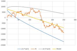
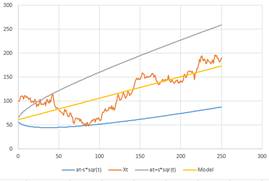
For our examples, we generate a simulated data using set of parameters drift $ m $ and volatility $ s $ , and initial value of the ABM, $ x_0 $. We consider this set of input as the true value of the parameters. Then we use the two steps calibration procedure above to estimate value of the parameters. The plot of the data and the model as well as the boundary of $ X_t=x_0+mt\pm s\sqrt{t} $ shows that the model fit the data very well.

Figure below show two representations of our examples with the true parameters that generate the data and their estimations. Notice that the model is always a straight line of the trend. The boundary is larger over time to show that the accuracy of prediction is lower by longer time from now.