Parameter Estimation of Geometric Brownian Motion

Share this: Google+
< Previous | Contents | Next >

Parameters Estimation in GBM

Suppose you have historical price data and you want to use Geometric Brownian motion model. How are you going to get the parameters of drift $ \mu $ and volatility $ \sigma $?

Recall GBM model is

$$ X_t=x_0 e^{(\mu-\frac{1}{2} \sigma^2) t+\sigma w_t } $$

where $ w_t \sim \sqrt{t} N(0,1) $. We input the Brownian motion, we have

$$ X_t=x_0 e^{(\mu-\frac{1}{2} \sigma^2) t+\sigma \sqrt{t} N(0,1) } $$

If we cannot use regression model directly because of the stochastic term $ N(0,1) $. Similar to the calibrating of ABM model, we can use two steps process to calibrate GBM model.

Step 1. Assume $ \sigma=0 $ to make GBM a deterministic model

$$ X_t=x_0 e^{\mu t} $$

This model can be easily transformed into a linear model by taking natural logarithm to both side of the equation

$$ \ln X_t =\ln x_0 + \mu t $$

Where the slope is equal to $ \mu $ and the intercept is equal to $ \ln x_0 $ . Note that

$$ x_0=e^{intercept} $$

Step 2. Using the parameter $ \mu $ that has been found in step 1 as a constant, we calculate the value of parameter $ \sigma $. In this second step, we only want to know the variation, not the mean. In this case, we can focus only on the standard deviation of $N(0,1) $ which is 1.

Let

$$ Z_t= \ln \frac{X_t}{x_0} = \tilde{\mu} t + \sigma w_t = (\mu -\frac{1}{2} \sigma^2) t+\sigma \sqrt{t} $$

In this case we have a quadratic equation in $ \sigma $, that is

$$ \frac{1}{2} t \sigma^2 - \sigma \sqrt{t} + (Z_t -\mu t)=0 $$

The positive solution of the quadratic equation is

$$ \sigma=-\frac{1}{2} + \frac{\sqrt{t-2t(Z_t-\mu t)}}{2 \sqrt{t}} $$

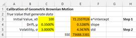
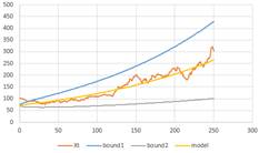
For our examples, we generate a simulated data using set of parameters drift $ \mu $ and volatility $ \sigma $ , and initial value of the GBM, $ x_0 $. We consider this set of input as the true value of the parameters. Then we use the two steps calibration procedure above to estimate value of the parameters. The plot of the data and the model as well as the boundary of $ X_t=x_0 e^{(\mu-\frac{1}{2} \sigma^2 )t\pm \sigma \sqrt{t} } $ shows that the model fit the data very well.

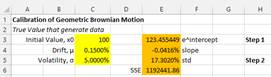
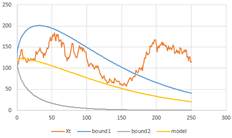
Figure below shows a representation of our examples with the true parameters that generate the data and their estimations. Observe that the estimated model is not linear. The boundary is larger over time to show that the accuracy of prediction is lower by longer time from now. In the second example in the right figure below, the estimated boundary does not always cover the data.