Arrival Distribution

< Previous | Next | Contents >

Arrival Distribution

This is the demand side of your queuing system. Arrival distribution represents the customers arrival into your system.

In most queuing system, at a given period of observation time, say for 12 hours of survey, the customers usually arrive randomly. The arrival of one customer is also independent from the arrival from other customers. They do not make agreement that one customer will arrive first, and then exactly 7 seconds later the next customer will arrive.

During the 12 hours of observational survey, usually we take, say, 5 minute period for one slot of observation. Then we set an observation line far behind the ordinary waiting line to count the number of customers arrive within the five minute observation. Table below shows an example of observation results from one cashier in a supermarket. If you have more than one cashier, the same observation and computation below need to be performed for each cashier.

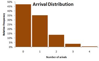
Once we obtain the data on the number of arrival, we can draw a distribution. Arrival distribution represents how many times we observe certain number of customers arrive within 5 minutes observation. Table below shows the count from the 12 observations and its relative frequency. The relative frequency is calculated based on the count and the total. For instance, for the second row 255/539*100% = 47%.

From the table above, we can draw the arrival distribution. This distribution is called probability mass function (PMF) because the number of arrivals is discrete.

The arrival rate in that cashier is computed as follow

0*47% + 1*35% + 2*13% + 3* 4% + 4*1% = 0.74768, rounded to 0.75.

We use notation lambda to indicate arrival rate, thus \( \lambda = 0.75 \) customers/5 minutes.

Most common type of arrival distribution of customers in a queuing system is random that follow Poisson Process or sometimes is called as Markovian. Using Chi-square goodness of fit, one can verify that the above example arrival distribution follows Poisson distribution.

Poisson distribution has formula for probability of x arrivals in a specific time period

$$ P(x) = \frac{\lambda^{x}e^{-\lambda}}{x!}, x=0,1,2,... $$

Where, \( \lambda \) is the arrival rate. Table below shows the probability based on Poisson distribution formula above. Notice that the theoretical probability of Poisson Distribution is very close to the relative frequency of our observation.

Note from statistical theory said that if the number of arrival in a given period of time occurs randomly and independently from other arrivals and follows a Poisson distribution with mean \( \lambda \) customers/minute, then the inter-arrival time (headway) distribution follow an exponential probability distribution with mean 1/\( \lambda \) minutes.

< Previous | Next | Contents >

Do you have queuing problem? Ask your expert for a solution here

These tutorial is copyrighted .

Preferable reference for this tutorial is

Teknomo, Kardi. (2014) Queuing Theory Tutorial
http://people.revoledu.com/kardi/tutorial/Queuing/